Linearization

General model of dynamic systems, please see Dynamic Systems.

Linearizing at arbitrary Equilibrium Point

Given:

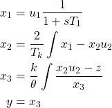
$\begin{align*}x_1&= u_1 \frac{1}{1+sT_1}\\x_2&=\frac{2}{T_k} \int{x_1-x_2u_2}\\x_3&=\frac{k}{\theta} \int \frac{x_2 u_2 - z}{x_3}\\y &= x_3\end{align*}$

Goal: Find

$\begin{align*}\dot{\mathbf{x}} + \Delta \dot{\mathbf{x}} =\mathbf{f}(\mathbf{x, u}, z) + \mathbf{A}\Big|_{\mathbf{x}^*, \mathbf{u}^*} \Delta \mathbf{x}+ \mathbf{B}\Big|_{\mathbf{x}^*, \mathbf{u}^*} \Delta \mathbf{u} + \mathbf{E}\Big|_{\mathbf{x}^*, \mathbf{u}^*} z\\ y = \mathbf{C}\Big|_{\mathbf{x}^*, \mathbf{u}^*} \Delta \mathbf{x}+ \mathbf{D}\Big|_{\mathbf{x}^*, \mathbf{u}^*} \Delta \mathbf{u} + \mathbf{F}\Big|_{\mathbf{x}^*, \mathbf{u}^*} z\\\end{align*}$

where $\mathbf{A}$ is the system matrix, $\mathbf{B}$ is the input matrix, $\mathbf{C}$ is the output matrix, $\mathbf{D}$ is the feedforward matrix, and $\mathbf{E}$ and $\mathbf{F}$ are noise matrices.

Step 1: Find state derivatives

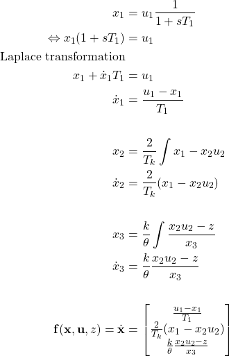
$\begin{align*}x_1&= u_1 \frac{1}{1+sT_1}\\\Leftrightarrow x_1 (1+ sT_1) &= u_1\\\text{Laplace transformation}&\\x_1 + \dot{x}_1 T_1 &= u_1\\\dot{x}_1 &= \frac{u_1 - x_1}{T_1}\\\\x_2&=\frac{2}{T_k} \int{x_1-x_2u_2}\\\dot{x}_2 &= \frac{2}{T_k} (x_1-x_2u_2)\\\\x_3&=\frac{k}{\theta} \int \frac{x_2 u_2 - z}{x_3}\\\dot{x}_3&=\frac{k}{\theta} \frac{x_2 u_2 - z}{x_3}\\\\\mathbf{f} (\mathbf{x},\mathbf{u}, z) = \dot{\mathbf{x}} &= \begin{bmatrix} \frac{u_1 - x_1}{T_1}\\ \frac{2}{T_k} (x_1-x_2u_2)\\\frac{k}{\theta} \frac{x_2 u_2 - z}{x_3} \end{bmatrix}\end{align*}$

Step 2: Find state equilibrium

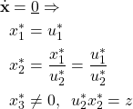
$\begin{align*}\dot{\mathbf{x}} &= \underline{0} \Rightarrow\\& x_1^* = u_1^*\\&x_2^* = \frac{x_1^*}{u_2^*} = \frac{u_1^*}{u_2^*}\\& x_3^* \neq 0, \hspace{2mm} u_2^* x_2^* = z\end{align*}$

Step 3: Linearization

$\begin{align*}&\mathbf{A} = \begin{bmatrix} \frac{\partial f_i}{\partial x_i} \end{bmatrix}, \hspace{2mm} \mathbf{B} = \begin{bmatrix} \frac{\partial f_i}{\partial u_i} \end{bmatrix}, \hspace{2mm} \mathbf{C} = \begin{bmatrix} \frac{\partial y}{\partial x_i} \end{bmatrix},\\&\mathbf{D} = \begin{bmatrix} \frac{\partial y}{\partial u_i} \end{bmatrix}, \hspace{2mm} \mathbf{E} = \begin{bmatrix} \frac{\partial f_i}{\partial z} \end{bmatrix}, \hspace{2mm} \mathbf{F} = \begin{bmatrix} \frac{\partial y}{\partial z} \end{bmatrix}\end{align*}$

State-space representation:

$\begin{align*}\dot{\mathbf{x}} + \Delta \dot{\mathbf{x}} &= \mathbf{f}(\mathbf{x, u}, z) + \mathbf{A}\Big|_{\mathbf{x}^*, \mathbf{u}^*} \Delta \mathbf{x}+ \mathbf{B}\Big|_{\mathbf{x}^*, \mathbf{u}^*} \Delta \mathbf{u} + \mathbf{E}\Big|_{\mathbf{x}^*, \mathbf{u}^*} z\\\Delta \dot{\mathbf{x}} &= \begin{bmatrix} -\frac{1}{T_1} & 0 & 0\\ \frac{2}{T_k} & - \frac{u_2}{T_k} & 0 \\ 0 & \frac{k}{\theta} \frac{u_2}{x_3} & -\frac{k}{\theta} \frac{x_2 u_2 - z}{x_3^2}\end{bmatrix}\Bigg|_{\mathbf{x}^*, \mathbf{u}^*} \Delta \mathbf{x} + \begin{bmatrix} -\frac{1}{T_1} & 0\\ 0 & - \frac{2}{T_k} x_2\\ 0 & \frac{k}{\theta} \frac{x_2}{x_3}\end{bmatrix}\Bigg|_{\mathbf{x}^*, \mathbf{u}^*} \Delta \mathbf{u} + \begin{bmatrix} 0 \\ 0 \\ -\frac{k}{\theta} \frac{1}{x_3} \end{bmatrix}\Bigg|_{\mathbf{x}^*, \mathbf{u}^*} \Delta z\\& = \begin{bmatrix} -\frac{1}{T_1} & 0 & 0\\ \frac{2}{T_k} & - \frac{u_2^*}{T_k} & 0 \\ 0 & \frac{k}{\theta} \frac{u_2^*}{x_3^*} & 0 \end{bmatrix} \Delta \mathbf{x} + \begin{bmatrix} -\frac{1}{T_1} & 0\\ 0 & - \frac{2}{T_k} x_2^*\\ 0 & \frac{k}{\theta} \frac{x_2^*}{x_3^*}\end{bmatrix} \mathbf{u} + \begin{bmatrix} 0 \\ 0 \\ -\frac{k}{\theta} \frac{1}{x_3^*} \end{bmatrix} \Delta z\\y&= \begin{bmatrix} 0 & 0 & 1\end{bmatrix} \mathbf{x}\end{align*}$

Linearizing along a Reference Trajectory

Given:

$\begin{align*}m\ddot{z} + a \dot{z}^2 &= u(V-\dot{z}), \hspace{3mm} z, \dot{z} \geq 0, \hspace{3mm} V, a: \text{constants} > 0\\y &= \ddot{z}\end{align*}$

Step 1: Find state space representation

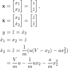
$\begin{align*} \mathbf{x} &= \begin{bmatrix} x_1 \\ x_2 \end{bmatrix} = \begin{bmatrix} z \\ \dot{z} \end{bmatrix},\\\dot{\mathbf{x}} &=\begin{bmatrix} x_2 \\ \dot{x}_2 \end{bmatrix} = \begin{bmatrix} \dot{z}\\ \ddot{z} \end{bmatrix} \\{y} &= \ddot{z} = \dot{x}_2\\ \dot{x}_1 &= x_2 = \dot{z}\\ \dot{x}_2 &= \ddot{z} = \frac{1}{m}(u(V-x_2) - a x_2^2) \\ &= \frac{V}{m} u- \frac{1}{m}ux_2 - \frac{a}{m}x_2^2 \end{align*}$

$\begin{align*} \mathbf{\dot{x}}&= \begin{bmatrix} x_2\\ \frac{V}{m} u- \frac{1}{m}ux_2 - \frac{a}{m}x_2^2 \end{bmatrix}\\ {y}&= \frac{V}{m} u- \frac{1}{m}ux_2 - \frac{a}{m}x_2^2 \\\end{align*}$

Step 2: Find linearized state space representation

$\begin{align*} \Delta \mathbf{\dot{x}} &= \begin{bmatrix} 0 & 1\ \\ 0 & -\frac{1}{m}(2ax_2^* + u^*) \end{bmatrix} \Delta \mathbf{x} + \begin{bmatrix} 0\\ \frac{1}{m}(V-x_2^*) \end{bmatrix} \Delta u \\y &= \begin{bmatrix} 0 & -\frac{1}{m}(2ax_2^* + u^*) \end{bmatrix} \Delta \mathbf{x}+ \frac{1}{m}(V-x_2^*) \Delta u\end{align*}$

Step 3: Use given reference trajectory to define the optimal state and input
Given: Reference trajectory $z(t)$ , starting from $A$ to target $B$ with $z^A = 0$ and $z^B=2$

$\begin{align*} z(t) = z^A + \frac{z^B - z^A}{2}(1- \cos({\Omega t})) & & 0\leq t \leq \frac{\pi}{\Omega}. \end{align*}$

After inserting $z^A$ and $z^B$ , we obtain $z(t) = 1- \cos(\Omega t)$

Now, we use the state representation:

$\begin{align*}\mathbf{x} = \begin{bmatrix}z\\\dot{z}\end{bmatrix}\end{align*}$

We obtain the optimal state:

$\begin{align*} \mathbf{x}^*(t) = \begin{bmatrix}1-\cos(\Omega t) \\\Omega \sin(\Omega t)\end{bmatrix}\end{align*}$

Now, we want to find the optimal input of the system

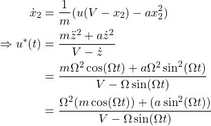
$\begin{align*}\dot{x}_2 &= \frac{1}{m}(u(V-x_2) - a x_2^2)\\\Rightarrow u^*(t) &= \frac{m\ddot{z}^2 +a \dot{z}^2}{V-\dot{z}}\\&= \frac{m \Omega^2\cos(\Omega t)+ a \Omega^2 \sin^2(\Omega t) }{V- \Omega \sin(\Omega t)} \\&= \frac{\Omega^2 (m \cos(\Omega t))+(a \sin^2(\Omega t))}{V-\Omega \sin(\Omega t)}\end{align*}$

Step 4: Insert optimal values in to the linearized state space representation

$\begin{align*} \Delta \mathbf{\dot{x}} &= \begin{bmatrix} 0 & 1\\ 0 & -\frac{(2a \Omega \sin(\Omega t))}{m} + \frac{\Omega^2 (m \cos(\Omega t))+(a \sin^2(\Omega t))}{V-\Omega \sin(\Omega t)} \end{bmatrix} \Delta \mathbf{x} + \begin{bmatrix} 0 \\ \frac{V- \Omega \sin(\Omega t)}{m} \end{bmatrix} \Delta u \\ y &= \begin{bmatrix} 0 & -\frac{(2a \Omega \sin(\Omega t))}{m} + \frac{\Omega^2 (m \cos(\Omega t))+(a \sin^2(\Omega t))}{V-\Omega \sin(\Omega t)} \end{bmatrix} \Delta \mathbf{x} + \frac{1}{m}(V- \Omega \sin(\Omega t)) \Delta u \end{align*}$

Linearizing at arbitrary Equilibrium Point

Linearizing along a Reference Trajectory

Neueste Beiträge

Neueste Kommentare